Besides computer vision, artificial neural networks (ANNs) are also very popular in natural language processing. Automatic translation or sentiment analysis of reviews are well known areas, where (recurrent) neural networks are used a lot. Around natural language understanding, there are even more applications. I want to show how to use neural networks for dialog classification.
Use cases
A dialog is a conversation between two participants in textual form (what´s app chats, booking, reservation…). There a lot of beneficial use cases, where extracted information of these dialogs can be valuable. You could simply get information about if the dialog was successful in terms of a reservation or transaction. You could classify a dialog into topics and so on.
When using ANNs for such a task at some point you might ask how to represent the dialog structure in the network architecture to get the best results. There are a lot of examples how to build ANNs for sentiment analysis and simple text classification, but dialogs are kind of different. Treat a dialog as a document works but does not really work very well. How to build a architecture for this kind of data is what I will try wo explain here.
Data
For all these use cases data is necessary to train a machine learning system and these data must be annotated with labels. The problem for a successful reservation is a binary classification of chat-like text data, where the training dataset consists of messages and these messages belong to threads.
Example:
Let’s assume the conversation is about finding a location for a meeting and we want to predict if the meeting happened.
Example of negative class (False Label).
| Number | Message | Expected prediction |
| #1 | Hello Linda, I would like to schedule a meeting for tomorrow after lunch. | 0.4 |
| #2 | Hi Sam, sure! Where do we want to meet? 1pm should be fine. | 0.7 |
| #3 | I have booked the meeting room in building 12, Room 43. | 0.8 |
| #4 | Ok perfect, see you there! | 0.9 |
| #5 | Hey Linda, unfortunately I am not ablte to attend today. I’ll contact you later on. | 0.4 |
Example of positive class (True Label).
| Number | Message | Expected prediction |
| #1 | Hi Alex, how are you? Do you have time tomorrow to talk about the remaining project? | 0.3 |
| #2 | Hi Sarah, sure let meet at 10:00 in the cafeteria. | 0.7 |
| #3 | Awesome, see you there. | 0.8 |
| #4 | Thanks for your feedback, I’ll consider to make it clear. | 0.9 |
Each thread is labeled with TRUE, if the conversation ended up in a meeting, but soemtimes it happens that in the last messages the meeting is canceld, so everything seems like this is a “1” until there.
The most challenging part of this classification task is that we want to predict the label of the thread at any state of the conversation. So, at some point in the conversation, it might be probable that the they meet, but in the last message one of them declines the meeting. This case should be predicted as well.
Baseline
To get a rough understanding what is possible with traditional approaches it is always a good idea to use these approaches as a baseline for further experiments.
One common approach to for text classification is to transform our text into some simple Bag-of-Words representation and use a support vector machine for classification. Additional it is necessary to preprocess the text data. Therefore, the data is cleaned, filtered by stop words and stemming is applied. All of these steps can be done in sci-kit learn with very little effort (example benchmark script).
Recurrent neural networks
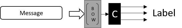
Using the same bag of words approach in neural networks seems to be an option, but does BoW really work for such a use case? Is it enough to just look at the words contained in the dialog, without respecting the word order or even, which participant wrote this word?
Well no obviously not, applying ANNs on instead of SVMs does not improve performance here. We should preserve as much as information as possible in the data. Word embeddings are the way to go. Word embeddings represent a word in semantic space, which means the word is represented as a vector by its meaning. Now our dialog is modeled as a sequence of words. Still there is no information about, who wrote the message but at least we have a word order.
Word embeddings and stacked recurrent neural networks
Word embeddings like word2vec, Glove and fastText are well known in natural language processing. With these embeddings we represent words as fixed size vectors and therefore a sentence is a sequence of word embeddings. Sequences are more complicated, due their variable length, but they have a major advantage, which is the order of the words.
To deal with sequences we use recurrent neural networks. There are several different RNNs, but the most successful ones are LSTMs and GRUs.
This is were the coding starts. To define a RNN in Keras we define a model like this:
model = Sequential()
model.add(Embedding(num_features, output_dim=32, input_length=seq_length))
model.add(LSTM(32, return_sequences=True, input_shape=(seq_length,32)))
model.add(LSTM(32, return_sequences=True))
model.add(LSTM(32))
model.add(Dense(1, activation='sigmoid'))
model.compile('adam', 'binary_crossentropy', metrics=[matthews_correlation, 'accuracy'])
But what does it actually mean?
Let´s start with the first line. We use a sequential model, which is easier but less powerful then functional models, which we use later. The first layer is the embedding layer, which is in our case the layer which takes word indices and transforms these indices to a vector representation. In this case we learn the embeddings from scratch, but it would be possible to use pretrained embeddings with the usage of:
model.add(Embedding(num_features, output_dim=32, input_length=seq_length, weights=[embedding_matrix], trainable=False))
Another option would be to use pretrained initial embedding but make them trainable.
The stacked LSTM layers are responsible to learn the internal states. The difference in these three layers is return_sequences, which is necessary if we want to stack the recurrent layers. With return_sequences set to True the LSTM returns the internal state for each timestep, if it is set to False it does only return the last value. In the last LSTM we only want to know the result without having to address any sequence data, for every cell we only got the result. All of these cell results are now used in the last layer, which is just one single neuron and this neuron makes the final classification. Compiling the model is the last step. Adam is the optimizer used, binary_crossentropy is the loss metric and metrics should be clear.
Attention decoder
Lets try to improve the results with attention mechanism, which is used in seq2seq applications, but should be useful here too. Attention is basically a mechansim, which learns what part of the text is more imporant then the others in a specific context. The implementation of the Attention decoder can be found here.
model = Sequential()
model.add(Embedding(num_features, output_dim=embedding_dim, input_length=seq_length))
model.add(LSTM(32, input_shape=(seq_length, embedding_dim), return_sequences=True))
model.add(AttentionDecoder(32, embedding_dim))
model.add(LSTM(32))
model.add(Dense(1, activation='sigmoid'))
model.compile('adam', 'binary_crossentropy', metrics=[matthews_correlation, 'accuracy'])
Bidirectional recurrent layers
Another option to improve the model, is to not only look at previous word in the sentence, but to look at the following words. This is called bidirectional LSTM and is simply implemented by having basically two RNNs cells, one for forward direction and one for the backward path. In Keras we can just add the Bidirectional layer wrapper.
model = Sequential()
model.add(Embedding(num_features, embedding_dim, input_length=seq_length))
model.add(Bidirectional(LSTM(32, dropout=0.3, recurrent_dropout=0.3, kernel_regularizer=regularizers.l2(0.01), return_sequences=True)))
model.add(AttentionDecoder(32, embedding_dim))
model.add(Bidirectional(LSTM(32, dropout=0.3, recurrent_dropout=0.3, kernel_regularizer=regularizers.l2(0.01))))
model.add(Dense(1, activation='sigmoid'))
model.compile('adam', 'binary_crossentropy', metrics=[matthews_correlation, 'accuracy'])
Regularization and dropout
You may notice a difference in the last snippet. With dropout and regularization added to our layers, we can avoid overfitting, while training. Regularization just adds a term to the cost metric, which penalizes large values (exploding gradients) and dropout is used to avoid, that single neurons become to important for the network. It makes the network more reliable, but on the other hand often increases the number of epochs necessary.
Convolution networks
Now there is another popular approach to solve the text classification problem, which is quite different from the previous ones. In this sequential convolution approach, we make use of convolutional layers, which are mostly applied in computer vision.
To understand how it works, there is a very good blog post about convolution in NLP. With this more complex architecture we can make use of the functional model definition, which is more powerful.
nlp_input = Input(shape=(seq_length,), name='nlp_input')
emb = Embedding(output_dim=embedding_size, input_dim=num_features, input_length=seq_length)(nlp_input)
emb = Dropout(0.3)(emb)
c1 = Conv1D(32, 4, padding='valid', activation='relu', strides=1, kernel_regularizer=regularizers.l2(0.01))(emb)
p1 = GlobalMaxPooling1D()(c1)
c2 = Conv1D(32, 8, padding='valid', activation='relu', strides=1, kernel_regularizer=regularizers.l2(0.01))(emb)
p2 = GlobalMaxPooling1D()(c2)
c3 = Conv1D(32, 16, padding='valid', activation='relu', strides=1, kernel_regularizer=regularizers.l2(0.01))(emb)
p3 = GlobalMaxPooling1D()(c3)
x = concatenate([p1, p2, p3])
x = Dense(32, activation='relu')(x)
x = Dropout(0.3)(x)
x = Dense(1, activation='sigmoid')(x)
model = Model(inputs=nlp_input, outputs=x)
model.compile('adam', 'binary_crossentropy', metrics=[matthews_correlation, 'accuracy'])
In general, the sequential convolution does exactly work like the convolution in computer vision, with one difference. It only takes one dimension to go through, which is in our case the word sequence. One kernel is looking at 4 words at once, one is looking at 8 and one is looking and 16. For every kernel size there are 32 filters (word combinations) learned. Then max pooling is applied for each feature map and the results are concatenated together. After concatenation there is a dense layer for classification.
Hierarchical models
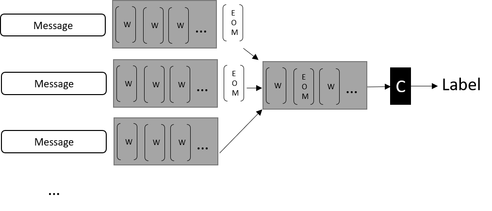
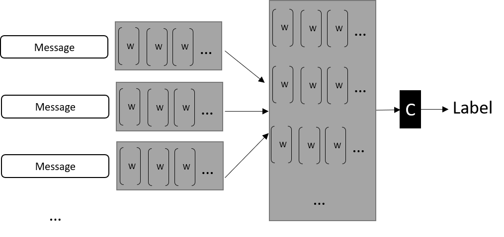
With some adjustments, it is possible to build a keras model, which can handle sequences of sequences of word embeddings. Every message consists of a sequences of word embeddings a thread consists of messages. To handle that, we can stack LSTMs.
nlp_seq = Input(shape=(number_of_messages ,seq_length,), name='nlp_input')
emb = TimeDistributed(Embedding(input_dim=num_features, output_dim=embedding_size,
                    input_length=seq_length, mask_zero=True,
                    input_shape=(seq_length, )))(nlp_seq)
msg_out = TimeDistributed(Bidirectional(LSTM(32)))(emb)
x = LSTM(32)(msg_out)
out = Dense(1, activation='sigmoid')(x)
model = Model(inputs=nlp_seq , outputs=out)
The most important layer here is the TimeDistributed layer. What it does is, to apply the inner layer (e.g. the embeddings layer) to every single timestep. The key point is, that the weights are shared, so you are using the same layer for every timestep. It is essentially doing the same as iterating through all timesteps and applying the layer to each of the timestep.
The input data has to be 2D for each sample or a 3D Tensor with (None, num_messages, seq_length) to make these kind of prediction . The embedding layer is converting the input data into some 4D tensor (None, num_messages, seq_lenght, embedding_size). Now the LSTM is appled for every message (TimeDistributed), which means it does create output of (num_messages, seq_lengh, 64). The 64 is the number of neurons (32) in the LSTM layer times two, because it is a bidirectional one (2 LSTMs, backward and forward pass and the output is concatenated). Now that we have an inner representation for every message, we can apply another LSTM onto the message sequence and finally get our result.
Using this architecture is quite heavy and needs a lot time to train. To make it faster, we could also go for convolutional instead of recurrent layers. Therefore, we just replace the second LSTM with 1D convolutions.
c1 = Conv1D(filter_size, kernel1, padding='valid', activation='relu'))(msg_out)
p1 = GlobalMaxPooling1D()(c1)
c2 = Conv1D(filter_size, kernel2, padding='valid', activation='relu')(msg_out)
p2 = GlobalMaxPooling1D()(c2)
c3 = Conv1D(filter_size, kernel3, padding='valid', activation='relu')(msg_out)
p3 = GlobalMaxPooling1D()(c3)
x = concatenate([p1, p2, p3])
The kernel size represents the number of messages to look at locally (“dependencies between messages”). The filter_size is the number of different filters (“dependency policies”).
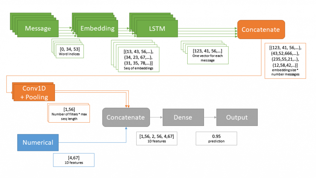
Adding metadata
It is even possible to add meta data (numerical) to the model, as described in the previous post.In this metadata the information about the author of each message can be stored and furthermore some other data can be attached.
Then we have a model, which looks as the following.
Training in practice
It is possible that you can train your network twice and get different results. This is a major problem with neuronal networks. Sometimes it is better to cancel training and restart, when the training does not work (random initialization).
To get reliable results first try to find hyperparameters with cross validation and grid search. This is already a problem because training takes too long to execute grid search on big datasets. Some people say Bayesian optimization is the solution, but I made better progress with grid search and a reduced cross validation with less folds and make several runs from coarse to fine. Hyperparameters include the network architectures, you can easily have hundreds of different parameters sets for your network.
If you include the number of epochs as a hyper parameter, it´s over. What I actually did is trying to train the network with a smaller dataset and train/test spilt to see if it converges and use early stopping in keras to speed up the training. Then I used the top N of these networks and executed a grid search with 3-fold cross validation (3 times for each param set), again with early stopping. For early stopping it is necessary to have a validation split inside of each cross-validation step. You don´t want to use early stopping with training scores, due overfitting.
Even this reduced approach takes a lot of time.


Request for dataset used in this article. You are referring to a dataset consisting of dialogue classification task. I am currently working on same task and would like to ask if you could send me this dataset for further analysis as it would help me verify our proposed system.
Hi Yang, sorry for that late reply, I was not checking for comments. The data set is not public and I can not share it, sorrry. Cheers Christian