In the last months I was working on a deep learning project. The goal was to dig into Tensorflow and deep learning in gerneral. For this purpose I re-implemented a paper from January 2016 called convolutional pose machines , which uses deep learning to predict human poses from images. Pose estimation is still an active research topic, due its very hard to solve. In this post i will try to give a short overview about this project. Github link here.
Frameworks
At the beginning I knew caffe and tensorflow, but just to note some others here is a list:
- Tensorflow (C++, Python)
- Caffe (C++, Python, MATLAB)
- Theano (Python)
- Torch (C++, Lua)
- Keras/Lasange (Python, built on top tensorflow/caffe)
- DeepLearning4J (Java, Scala, JVM, awesome documentation)
Read this post for more details.
Tensorflow seems to be the framework for cutting edge development and there is another library which makes usage of tensorflow easier called tensorpack.
Very basic deep learning introduction
Deep convolutional neural nets consist of three core components, which are stacked to an architecture depending on the task. These three components are called convolutional layer, pooling layer and fully connected layer. While the first two layers are combined, and are responsible for abstraction of features and generalization, the last layer is the classification layer, which puts the output from the other layers together and do the prediction. Basically, covNets work based on abstraction.
Convolutional layers
The convolutional layer is the name giving layer, which applies a convolutional kernel to images, extracting a feature. A feature is another representation of the original input and is used by the following layers as input.
A kernel is based on how the human brain works. The human brain processes images in snippets, which are called receptive fields. A kernel does define a region (e.g. 9×9) and only considers these areas for calculation, so it’s a local or neighborhood method. When a kernel is applied on an image, the kernel slides through the image, with a specified stride. If the kernel is an edge detector, the output image, would be an image of edges, where the edge is the feature, which was detected.
Several of these kernels are applied at the same time and the generated new “images” are called feature maps. The weights of the kernel are trained in the training phase and define the internal feature transformation for each of those feature maps. So if we take a raw input image and train the network with an label image, which was generated by an sobel edge detector the network will learn the sobel edge detector kernel weights itself, approximately.
Pooling
The pooling layer is the aggregating and generalizing layer. In the most cases a max pooling is proposed and this is what happens in this project too. Pooling does reduce the computation cost and increases the locally independence of features found, because it does provide a basic translation invariance.
Fully connected layer
The fully connected layer is often a layer with a 1×1 kernel. So technically there is no difference between convolutional and fully-connected layers, but the 1×1 sized kernel implies some more complexity.
The fully connected layer gathers all the features from previous layers and does the regression/classification, based on the most abstract features. Sometimes there are several of these layers in succession, to make the classifier more complex. Because of the layer is fully connected, which means that every neuron is connected to every other neuron and all these connections can be trained, this layer is usually responsible for the most of free parameters and subsequently the training duration.
Much better and deeper introduction here.
Data
Deep Learning is strongly restricted by the amount of existing data to train the covNet (convolutional neural network). To enable our network to predict poses in an image, we need a training dataset, which contains people and annotated positions. Furthermore, it is very important to find a data set, which is already big enough and free to use.
The MPII data set
The MPII data set consists of more than 25,000 images, which contain over 40,000 annotated persons and is designed for 2D pose estimation. This data was selected based on a taxonomy of 800 activities and contains 410 different activities, which are also part of the annotation. This data set was extracted from youtube videos and contains many different perspectives and occlusions.
The data is not preprocessed in any way, so aspect ratio and size is different for many of the images. To train a covNet, it is necessary to have equal sized images and try to get a person into the middle of the image. The first step was to preprocess the data. I don´t want to go into details here, you can look at the code, if you want to know more about it.
Problem
In the Mpii data set there are several images, which include more than one human. If the network is trained to predict 2D coordinates of the joint positions, there is the problem of training with multiple labels. If an image shows more than one single person, but the labels only mark the joints of one person, the network is told that there is only a single person. This would lead to bad performance. Thus, the common approach to solve this is to create an activation/confidence map. Confidence maps are basically images of feature probabilities. To transform the position labels to these activation maps the Gaussian normal distribution around the center label position is generated as an image. The network is trained to find a prediction image, which fits the training image (regression).
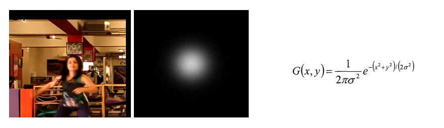
Here we can see the input image (l) and how the label image(m) looks like, calculated with the 2d gauss formula(r). The net is trained to learn this relation.
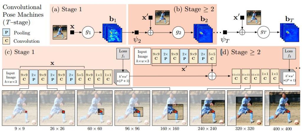
This image shows the network architecture from convolutional pose machines
Implementation
So the first step to is to implement the net architecture in tensorpack. This is surprisingly easy, but getting the framework running correctly is not, but this is a different story. This code is also inspired by the posemachines implementation in tensorpack, wich came up, while i was almost finished with my implementation.
I tried to explain the code in the comments, I recommend to go through the tensorflow/tensorpack documentation before trying to understand this code. (Note BODY_PART_COUNT is 16)
  def _build_graph(self, input_vars, is_training):
        # get image and label
        image, label = input_vars
        # generate a gaussian image from the label (translate a existing template image to achieve this)
        gaussian = gaussian_image(label)
        #define a tensor, which is shared across the graph (weights)
        shared = (LinearWrap(image)
                  # define the architecture almost like in the paper
                  # small difference the 9x9 layer is split into two 3x3 layers
                  .Conv2D('conv1_1', 64, kernel_shape=3)
                  .Conv2D('conv1_2', 64, kernel_shape=3)
                  .MaxPooling('pool1', 2)
                  # 184*184
                  .Conv2D('conv2_1', 128, kernel_shape=3)
                  .Conv2D('conv2_2', 128, kernel_shape=3)
                  .MaxPooling('pool2', 2)
                  # 92*92
                  .Conv2D('conv3_1', 256, kernel_shape=3)
                  .Conv2D('conv3_2', 256, kernel_shape=3)
                  .Conv2D('conv3_3', 256, kernel_shape=3)
                  .Conv2D('conv3_4', 256, kernel_shape=3)
                  .MaxPooling('pool3', 2)
                  # 46*46
                  .Conv2D('conv4_1', 512, kernel_shape=3)
                  .Conv2D('conv4_2', 512, kernel_shape=3)
                  .Conv2D('conv4_3_CPM', 256, kernel_shape=3)
                  .Conv2D('conv4_4_CPM', 256, kernel_shape=3)
                  .Conv2D('conv4_5_CPM', 256, kernel_shape=3)
                  .Conv2D('conv4_6_CPM', 256, kernel_shape=3)
                  .Conv2D('conv4_7_CPM', 128, kernel_shape=3)())

        # each stage is refining the confidence map of each body part
        def add_stage(stageNum, prev):
            # here the shared network part is re-used and combined with the previous stage
            prev = tf.concat(3, [prev, shared])
            # six refinement stages
            for i in range(2, 7):
                prev = Conv2D('Mconv{}_stage{}'.format(i, stageNum), prev, 128, kernel_shape=7)
            prev = Conv2D('Mconv6_stage{}'.format(stageNum), prev, 128, kernel_shape=1)
            prev = Conv2D('Mconv7_stage{}'.format(stageNum), prev, BODY_PART_COUNT, kernel_shape=1, nl=tf.identity)
            # reorder the data
            pred = tf.transpose(prev, perm=[0, 3, 1, 2])
            pred = tf.reshape(pred, [-1, 46, 46, 1])
            #squared error for each stage
            error = tf.squared_difference(pred, gaussian, name='se_{}'.format(stageNum))
            return prev, error

        # the first one is different
        belief = (LinearWrap(shared)
                  .Conv2D('conv5_1_CPM', 512, kernel_shape=1)
                  .Conv2D('conv5_2_CPM', BODY_PART_COUNT, kernel_shape=1, nl=tf.identity)())
        # error calculation
        se_calc = tf.transpose(belief, perm=[0, 3, 1, 2])
        se_calc = tf.reshape(se_calc, [-1, 46, 46, 1])
        error = tf.squared_difference(se_calc, gaussian, name='se_{}'.format(1))

        # stack the stages
        for i in range(2, 7):
            belief, e = add_stage(i, belief)
            error = error + e

        # this is the result (confidence map for each body part)
        belief = tf.image.resize_bilinear(belief, [368, 368], name='belief_maps_output')
        # the mean squared error as cost metric
        cost = tf.reduce_mean(error, name='mse')
        # add l2 regularization against overfitting
        wd_cost = tf.mul(0.000001,
                         regularize_cost('conv.*/W', tf.nn.l2_loss),
                         name='wd_cost')
        # show costs in tensorboard
        add_moving_summary(cost, wd_cost)
        # show weights in tensorboard
        add_param_summary([('.*/W', ['histogram'])])  # monitor W
        # define the cost term
        self.cost = tf.add_n([cost, wd_cost], name='cost')
Validation
At the moment there is the cost metric, which defines the error of the training data, but we need a better validation metric. A popular metric ist the PCP (percentage of correct parts) metric. I used a very simple form of this metric, which does consider a body part as correct predicted if the coordinates are inside a 25 pixel radius of the ground truth.
        # python reshape magic (i really don´t like it)
        pred_collapse = tf.reshape(se_calc, [-1, 46 * 46])
        # find the max in each confidence map
        flatIndex = tf.argmax(pred_collapse, 1, name="flatIndex")
        predCordsX = tf.reshape((flatIndex % 46) * 8, [-1, 1])
        predCordsY = tf.reshape((flatIndex / 46) * 8, [-1, 1])
        predCordsYX = tf.concat(1, [predCordsY, predCordsX])
        predCords = tf.cast(tf.reshape(predCordsYX, [-1, 16, 2]), tf.int32, name='debug_cords')
        # the distance between label and prediction
        euclid_distance = tf.sqrt(tf.cast(tf.reduce_sum(tf.square(
            tf.sub(predCords, label)), 2), dtype=tf.float32), name="euclid_distance")
        # very simple pcp metric (radius of 25 pixel)
        minradius = tf.constant(25.0, dtype=tf.float32)
        incircle = 1 - tf.sign(tf.cast(euclid_distance / minradius, tf.int32))
        pcp = tf.reduce_mean(tf.cast(incircle, tf.float32), name="train_pcp")
        # pcp tracking in tensorboard
        add_moving_summary(pcp)
        # There is a magic trick in tensorpack, just use the worng tensor, which is evaluated in the validation step
        wrong = tf.identity(1 - pcp, 'error')
Results
First let me say, my goal was not to improve the pose estimation results or get some comparable scores. I just wanted to get into deep learning with tensorflow and I had a very experienced phd candidate (Samuel), who helped me a lot. In short, it was a very exiting project, and also an exhausting one, because the training took long every time and if something in the code is wrong or missing, the learning crashes or the model learns nothing useful (I don´t had the training workstation at home or available over network). Anyway, here are the results:

The first row shows some results with only 2 stages active, while in the second row shows results with 6 stages. Not only in the labeled images, we can see the that 2 stages are not enough for such a complex problem. The costs also show, that there is not good conversion, when only 2 stages are active.
You can use the pagination to see the final results, with the validation metric.
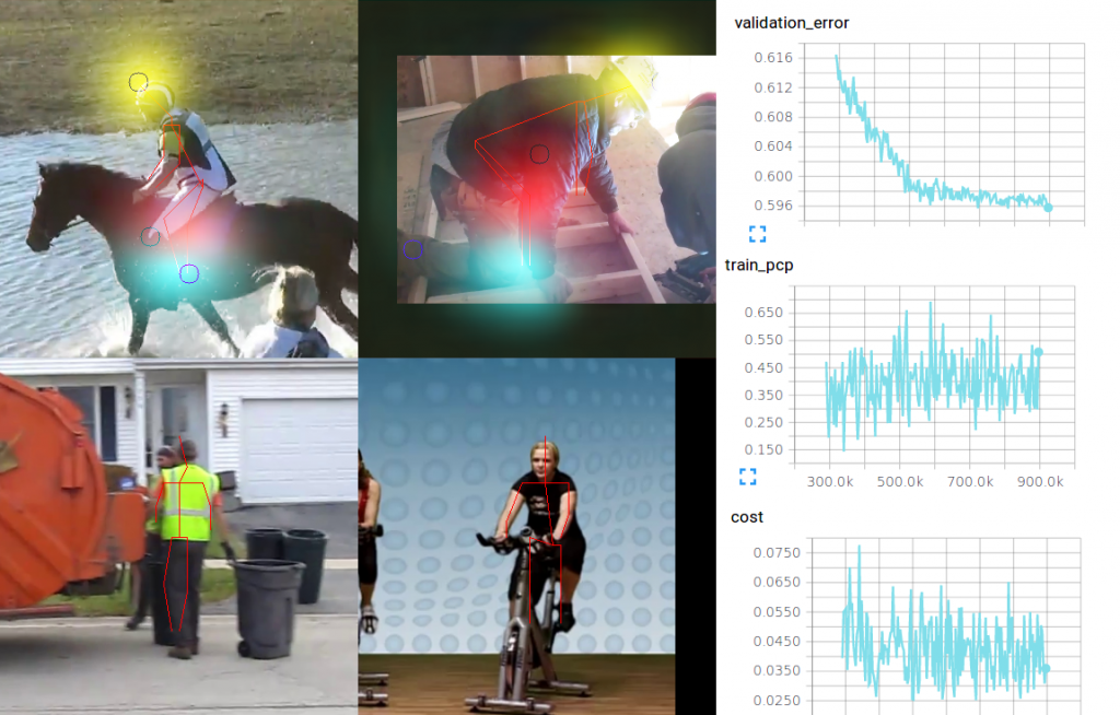
This are some examples from the final results. On the first row I overlayed 3 different confidence maps on very hard poses. The yellow one is the head, the red one the left knee and the blue is the right foot. We can see that the left pose estimation is ok, even with the occlusion and the right one is not very good at all.

I know this if off topic but I’m looking into starting my own blog and was curious what all is required to get setup? I’m assuming having a blog like yours would cost a pretty penny? I’m not very internet smart so I’m not 100% certain. Any suggestions or advice would be greatly appreciated. Kudos
I really like it when folks get together and share ideas. Great site, keep it up!
Nice work. Can post instructions on using your software? E.,g., conversion of the dataset, training, testing, and running the model?
Thanks,
Jay
Hi Jay,
you may want to take a look at this example
[…] a bit older, but if you are interested in deep learning for pose estimation, you might find this interesting. The post includes a small introduction to deep learning and how to deal with such a […]