In this post I would like to show how to use a pre-trained state-of-the-art model for image classification for your custom data. For this we utilize transfer learning and the recent efficientnet model from Google. An example for the standford car dataset can be found here in my github repository.
EfficientNet
Starting from an initially simple convolutional neural network (CNN), the precision and efficiency of a model can usually be further increased step by step by arbitrarily scaling the network dimensions such as width, depth and resolution. Increasing the number of layers used or using higher resolution images to train the models usually involves a lot of manual effort. Researchers from the Google AI released EfficientNet few months ago, a scaling approach based on a fixed set of scaling coefficients and advances in AutoML and other techniques (e.g. depth-wise-separable convolution, swish activation, drop-connect). Rather than independently optimizing individual network dimensions as was previously the case, EfficientNet is now looking for a balanced scaling process across all network dimensions.
With EfficientNet the number of parameters is reduces by magnitudes, while achieving state-of-the-art results on ImageNet.
Transfer Learning
While EfficientNet reduces the number of parameters, training of convolutional networks is still a time-consuming task. To further reduce the training time, we are able to utilize transfer learning techniques.
Transfer learning means we use a pretrained model and fine tune the model on new data. In image classification we can think of dividing the model into two parts. One part of the model is responsible for extracting the key features from images, like edges etc. and one part is using these features for the actual classification. Usually a CNN is built of stacked convolutional blocks reducing the image size while increasing the number of learnable features (filters) and in the end everything is put together into a fully connected layer, which does the classification. The idea of transfer learning is to make the first part transferable, so that it can be used for different tasks by replacing only the fully connected layer (often called “top”).
Implementation
This keras Efficientnet implementation (pip install efficientnet) comes with pretrained models for all sizes (B0-B7), where we can just add our custom classification layer “top”. With weights='imagenet' we get a pretrained model.
base_model = EfficientNetB5(include_top=False, weights='imagenet')
x = base_model.output
x = GlobalAveragePooling2D()(x)
predictions = Dense(num_classes, activation='softmax')(x)
model = Model(inputs=base_model.input, outputs=predictions)

# fix the feature extraction part of the model
for layer in base_model.layers:
    layer.trainable = False

model.summary()
Total params: 28,615,970
Trainable params: 102,450
Non-trainable params: 28,513,520
Now we can train the last layer on our custom data, while the feature extraction layers are using the weights from imageNet. But unfortunately we might see this results:
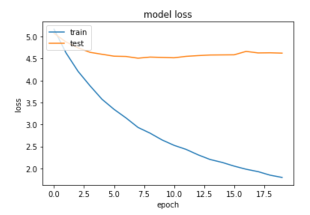
Training and testing loss, when freezing all layers from the pretrained model 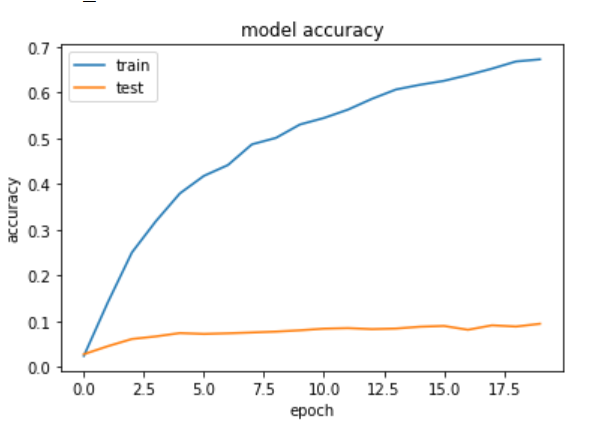
Training and testing accuracy, when freezing all layers from the pretrained model
The BatchNormalization weirdness
This weird behavior comes from the BatchNormalization layer. It seems like there is a bug, when keras (2.2.4) is running the validation in inference mode. However we could ignore this, because besides the weird validation accuracy scores, our layer still learns, as we can see in the training accuracy (Read more about different normalization layers here). But to fix it, we can make the BatchNormalization layer trainable:
for layer in base_model.layers:
    if isinstance(layer, BatchNormalization):
        layer.trainable = True
    else:
        layer.trainable = False
Unfortunately we loose the possibillty to use a larger batch_size, somehow keras seems to need much more memory when we make BatchNormaliation trainable. On the other hand we got reasonable results for validation:
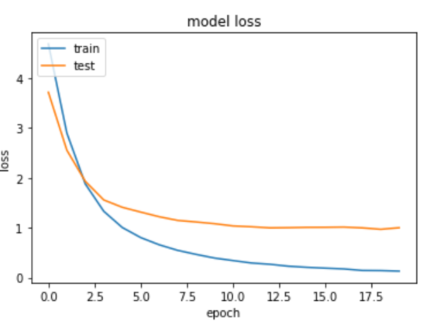
Training and testing loss, when unfreezing the BN layers from the pretrained mode 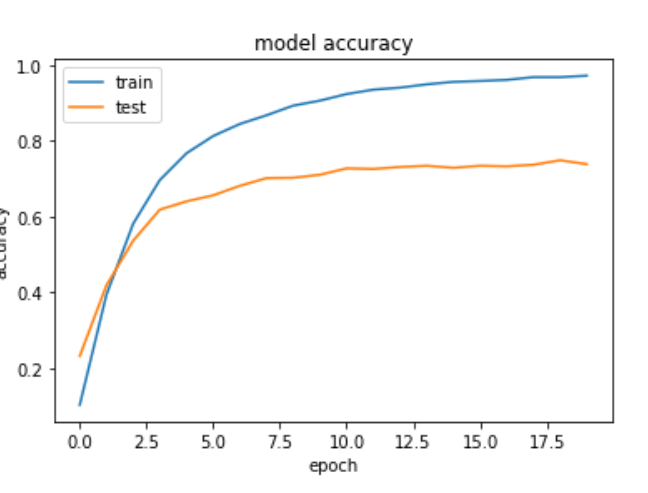
Training and testing accuracy, when unfreezing the BN layers from the pretrained mode
We still have additional benefits, when training the last layer(s) only. For example, we have less trainable parameters, which means faster computation time. But on large datasets, I would rather ignore the validation scores and take the advantages of the larger batch_size, by freezing the base model completly.
Release the full power of the network
At some point in the training progress, the model does not improve further and it’s time to open the rest of the network for fine-tune the feature extraction part. Therefore we make all the layers trainable and fit the model again.
for layer in model.layers:
    layer.trainable = True
model.summary()
Total params: 28,615,970
Trainable params: 28,443,234
Non-trainable params: 172,736
Caution: It’s important to avoid early overfitting of the model, because it can get hard for the model to escape the local minima, therefore we make sure to open the network better earlier then later for full training. Also, don’t forget to adjust the batch_size, or we run OOM. To get an estimate of the memory required by the model look here (stackoverflow). I also suggest making use of early stopping.
After running fit the second time, we just applied transfer learning.
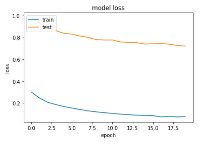
Training and testing loss for the full model 
Training and testing accuracy for the full model
Hint: To access the extracted features directly (not the labels) use the following code:
model_feature = Model(input=model.input, output=model.layers[-2].get_output_at(0))
predictions = model_feature.predict_generator(
    generator,
    steps=100,
    verbose=1)
[…] http://digital-thinking.de/keras-transfer-learning-for-image-classification-with-effificientnet/ […]
[…] http://digital-thinking.de/keras-transfer-learning-for-image-classification-with-effificientnet/ […]
[…] Recently, I wrote a post about the tools to use to deploy deep learning models into production depending on the workload. In this post I will show in detail how to deploy a CNN (EfficientNet) into production with tensorflow serve, as a part of TFX. The starting point here is a fine-tuned version of a keras model from here. […]